SPC Pipeline

Spatial Proximity based Clustering (SPC) is designed as a cell clustering strategy for spatial transcriptomics data which is free from pre-defined weight between expression and spatial. The model takes into account the functional and spatial proximity of cells to define hubs for cells in similar states or with similar functions. We do not provide novel clustering arithmetic but take advantage of published tools like Seurat and Scanpy.

Usage

The main workflow of SPC including:

• step1: define cell attributes, which you can do with clustering tools like Seurat or others you prefer

• step2: non-continuous segmentation on the spatial coordinate, which can be performed with our tools

• step3: re-clustering on the segmented spc cells

Example workflow:

preparation

import matplotlib.pyplot as plt
import anndata
import scanpy as sc
import spc

plot function to show annotation or clustering results on spatial

def spatial_plot(adata, color='annotation'):
  x, y = zip(*adata.obsm['spatial'])
  annotations = adata.obs[color].unique()
  colors = spc.colors[:len(annotations)]
  color_dict = dict((anno, color) for anno, color in zip(annotations, colors))
  c = [color_dict[anno] for anno in adata.obs[color]]
  plt.scatter(x, y, s=1, c=c, lw=0, edgecolors='none')
  plt.gca().set_aspect('equal')
  plt.show()

process function to cluster spatial data

def sc_pp(adata):
  sc.pp.normalize_total(adata)
  sc.pp.log1p(adata)
  sc.pp.highly_variable_genes(adata)
  sc.pp.scale(adata, max_value=10)
  sc.tl.pca(adata, svd_solver='arpack')
  sc.pp.neighbors(adata, n_neighbors=10, n_pcs=40)
  sc.tl.umap(adata)
  sc.tl.leiden(adata)

read in example data and make a copy for spc process

adata = anndata.read('mousebrain_cellbin.h5ad')
AnnData object with n_obs × n_vars = 50140 × 25879
  obs: 'annotation'
  var: 'Gene'
  uns: 'annotation_colors'
  obsm: 'spatial'
  layers: 'counts'

adata.X = adata.layers['counts']
adata.obs[['x', 'y']] = adata.obsm['spatial']
cell2coords = adata.obs[['x', 'y']].copy()
spc_adata = adata.copy()

view the original annotated celltype on spatial

spatial_plot(adata, color='annotation')

step1: first round of unsupervised clustering to generate cell attributes

sc_pp(adata)
spatial_plot(adata, color='leiden')

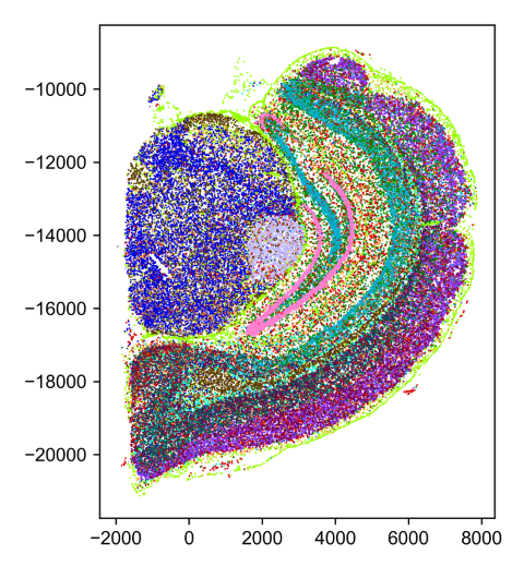
step2: perform SPC non-continuous segmentation based on the first round leiden clusters

perform spc non-continuous segmentation on original spc_adata and re-clustering on spc

 spc_adata.obs['leiden'] = adata.obs['leiden']
 spc_adata = spc.ncseg(spc_adata, celltype='leiden', meta_nCell=10, min_nCell=3)

... 0.02263174911089557   cells filtered for 0
... 0.008573928258967628  cells filtered for 1
... 0.018001125070316894  cells filtered for 2
... 0.01702890432444544   cells filtered for 3
... 0.03766963032288254   cells filtered for 4
... 0.016137040714995034  cells filtered for 5
... 0.01837270341207349   cells filtered for 6
... 0.023353967360720315  cells filtered for 7
... 0.02075187969924812   cells filtered for 8
... 0.0036258158085569255 cells filtered for 9
... 0.015986537652503154  cells filtered for 10
... 0.013006503251625813  cells filtered for 11
... 0.028044871794871796  cells filtered for 12
... 0.05420560747663551   cells filtered for 13

step3: second round of unsupervised clustering on spc cells

sc_pp(spc_adata)
spc_adata
 AnnData object with n_obs × n_vars = 5535 × 25879
   obs: 'leiden', 'cell_number', 'hood', 'x', 'y', 'min_radius', 'max_radius'
   var: 'Gene', 'highly_variable', 'means', 'dispersions', 'dispersions_norm', 'mean', 'std'
   uns: 'hvg', 'leiden', 'log1p', 'neighbors', 'pca', 'umap'
   obsm: 'X_pca', 'X_umap'
   varm: 'PCs'
   layers: 'counts'
   obsp: 'connectivities', 'distances'

visualization of SPC on deconvolved cells

plot function to show SPC clustering results
def spatial_plot_deconv(adata, cell2coords, color='annotation'):
  obs = adata.obs[['hood', color]].copy()
  obs['hood'] = obs['hood'].str.split(',')
  obs = obs.explode('hood').set_index('hood')
  obs = obs.merge(cell2coords, how='left', left_index=True, right_index=True)
  x = obs['x'].values
  y = obs['y'].values
  annotations = obs[color].unique()
  colors = spc.colors[:len(annotations)]
  color_dict = dict((anno, color) for anno, color in zip(annotations, colors))
  c = [color_dict[anno] for anno in obs[color]]
  plt.scatter(x, y, s=1, c=c, lw=0, edgecolors='none')
  plt.gca().set_aspect('equal')
  plt.show()

spatial_plot_deconv(spc_adata, cell2coords, color='leiden')

After you finish all these steps, you can easily compare results from different clustering methods.

Limited

The current version will drop cells which are failed to be assigned into any SPC (controlled by min_nCells parameters in spc.ncseg function).

Citation

Unpublished