Meta-Niche

This was used as the second part of co-localization estimation in our paper. For detailed information, see tutorial.

When considering niches, we always say surrounding cellular or molecular component of a target cell. However, focusing on only a single cell would never make sense in reference of any biology process, which prompt us to group cells with similar state and ask what elements may trigger the activate of this target cell group.

The following tutorial descibes a demo example for calculating surrounding cellular component of our target cell group c3, which represent neoblast cells in our paper. In this calculation, we used both distance and count of neighbor cells to infer the main ingredient of local microenvironment.

import pandas as pd
import niche
%matplotlib inline

we have included a demo file for testing, you can find with name ‘demo.txt’. In this file, each line represent a cell with its spatial coordinates x, y and cell categories cluster

df = pd.read_csv('demo.txt', sep='\t', header=0, index_col=0)
df

	x	y	cluster
cell
-23531.WT_25	2353.578947	1708.157895	c34
-23493.WT_25	2642.612903	1682.451613	c9
-23480.WT_25	2546.903226	1683.193548	c23
-23479.WT_25	2827.598726	1668.636943	c3
-23380.WT_25	2364.428571	1671.333333	c6
...	...	...	...
197449.WT_25	23.949495	754.535354	c18
197451.WT_25	22.048077	742.721154	c18
197454.WT_25	18.070796	707.345133	c18
197458.WT_25	16.148760	671.520661	c17
197460.WT_25	17.311688	747.246753	c18

61743 rows × 3 columns

as niches function in a local microenvironment, we first find neighbor cells of each neoblast cell (c3 group here) within radius of 15 um, and then relocated each neighbor’s coordinates by setting their query c3’s coordinates as origin point (0, 0), which reset the location of all c3 cells as a ‘meta’ representation and only retained neighbors’ relative position.

nce = niche.cal_niche(df, group='c3', group_col='cluster', radius=15)
nce

based on these relative positions, we next calculated the spatial density of each type of neighbors, and also estimated how close of each neighbor type to our c3 meta-coordinates.

results = niche.cal_2d_density(nce, group_col='cluster', radius=15)

/home/hankai/CodeSpace/4D-BioReconX/BIO/Meta-Niche/niche.py:149: UserWarning: Matplotlib is currently using module://matplotlib_inline.backend_inline, which is a non-GUI backend, so cannot show the figure.
  fig.show()

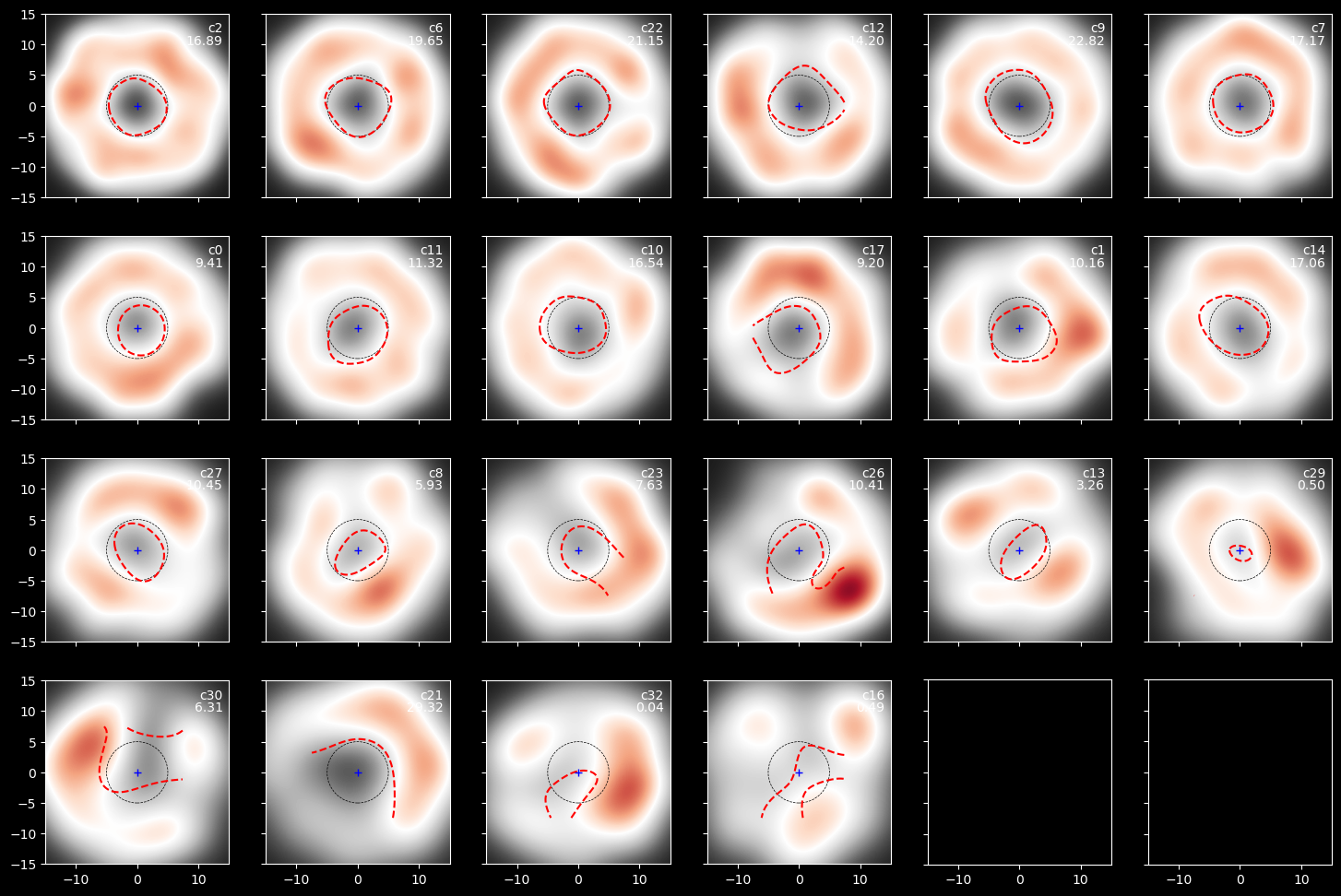
In each axis, the heatmap show the spatial density, with high density in red color. The blue cross in the middle represent the location of the meta-c3 (0, 0). The black-dotted circle represent a baseline with radius of 5 um, while the red-dotted circle represent the contour line with density of 0.001. The type of neighbor and the nearest distance of contour line to the (0, 0) was labeled at the upper-right corner.

results

	group	count	max_dens	nearest_dist
0	c2	2005	0.001833	16.892981
1	c6	865	0.001893	19.650777
2	c22	666	0.001836	21.152721
3	c12	568	0.001858	14.197462
4	c9	550	0.001718	22.821707
5	c7	491	0.001740	17.173243
6	c0	486	0.001809	9.406311
7	c11	375	0.001620	11.316524
8	c10	355	0.001631	16.539270
9	c17	326	0.001978	9.196763
10	c1	258	0.001980	10.156676
11	c14	230	0.001634	17.060274
12	c27	164	0.001833	10.452174
13	c8	151	0.001927	5.927211
14	c23	149	0.001828	7.633153
15	c26	138	0.002363	10.413944
16	c13	126	0.001800	3.258554
17	c29	101	0.002025	0.504831
18	c30	93	0.001979	6.310088
19	c21	93	0.001734	29.317459
20	c32	89	0.002039	0.040527
21	c16	64	0.001660	0.494309

The count of neighbors, as well as maximal density and nearest distance of each neighbor type were included in the final result

For custom usage

This method should work in any custom situations, but one thing to be aware of is that how your target cell groups distributed in space. Cell groups with scattered and aggregated distribution will be different.

Further extending

We designed this ‘meta’-based calculation as a preliminary steps, here we listed some possible directions as hints for future work and other people.

• 3D space coordinates

• additional conditions for spliting ‘meta’ into subtype, like region, state

• density polarity to find local response

• integrate with cell-cell communication